Ilastik Pixel Classification
Ilastik
Introduction
Ilastik is a software that leverages machine learning algorithms for image analysis tasks. The software is interactive and easy to use and no prior machine learning expertise is required.
Ilastik provides multiple workflows:
- Pixel classification
- Object classification
- Tracking
- Density counting
- Semi-manual 3D carving
This how-to guide is about pixel classification which is used for image segmentation. The user labels several regions in the image interactively with a brush tool. Based on the features of these labelled regions (intensity, gradient, etc.) the software then learns to predict the segmentation for the rest of the image. A random forest classifier is used in the background to learn the prediction from the labels.
For a full documentation of Ilastik please see the Online Ilastik Documentation.
Step-by-step
Prerequisite: Download and install Ilastik from here.
The example data for this guide is a series of 2D TEM images but the same steps can be applied to 3D data.
Step 1: Set up project
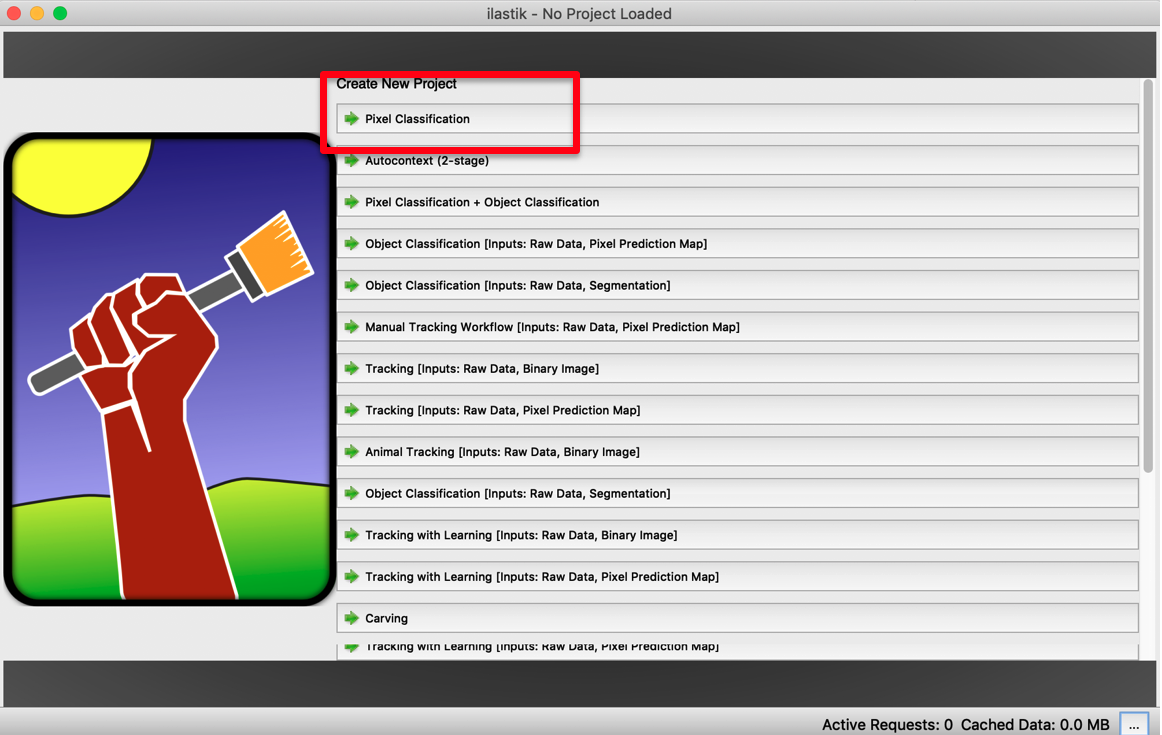
- Open Ilastik.
- Select: Create New Project > Pixel Classification.
- Save the project.
Step 2: Define input data
- Make sure Input Data tab is selected.
- (a) Drag & drop an image into the white area.
- (a) Alternative: Click Add New … > Add separate Image(s)…
This tutorial uses only one image for training but one can (and it is recommended) to add more images for training.
- (b) The image should appear in the list and be displayed.
- (c) Copy the image into your Ilastik project:
- Double-click the line with the image to open the Properties window.
- Under Storage, select Copy Into Project File.
- This menu also allows you to adjust more image properties (brightness, channels, …).
If your images are big don’t copy the data. Instead make sure that you keep your training images close to the project location (like in a subfolder).
(a)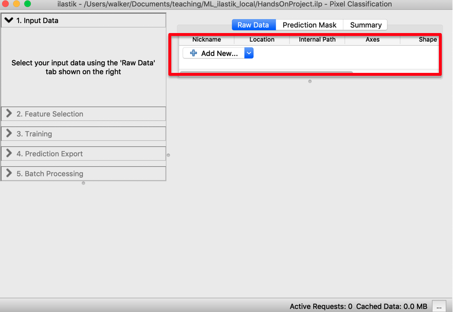 | (b)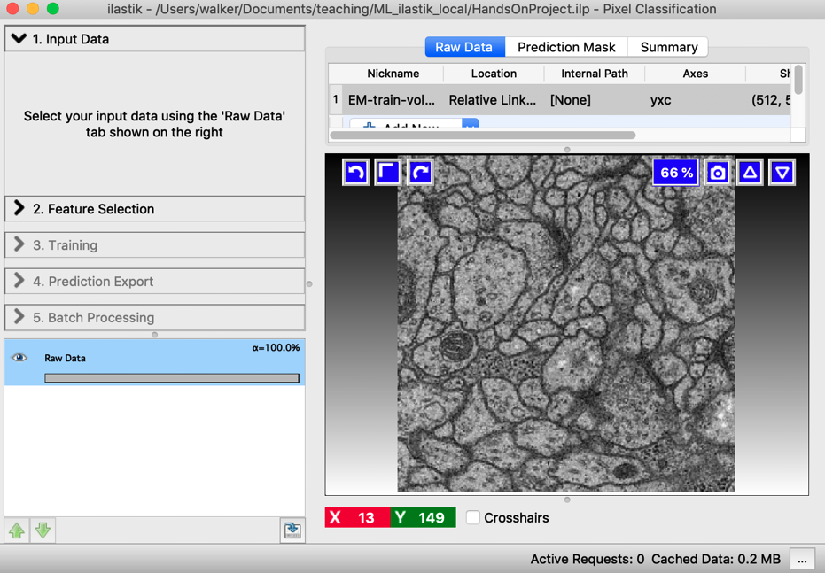 |
(c)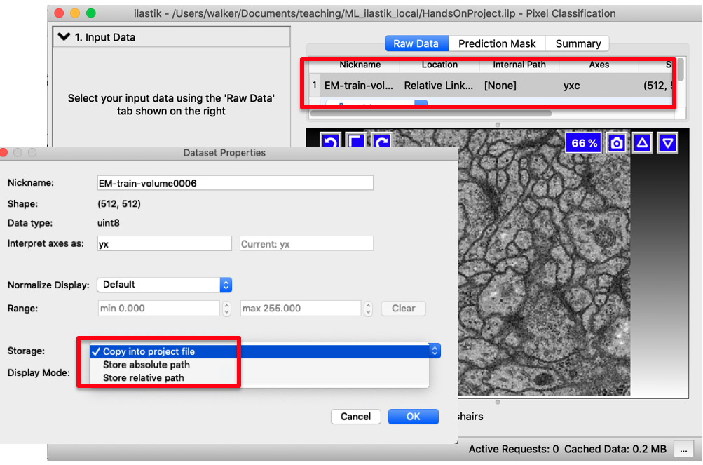 |
Step 3: Feature selection
- (a) Select Feature Selection tab.
- (a) Click on Select Features button.
- (a) Select a subset or all features.
Choose features from each category. The choice is initially a bit random and can be refined later.
The more features are selected, the longer the computation takes.
Larger sigma: detects bigger structures, but also computationally more expensive. - (b) Optional: Visualize the features: Visualization helps indicate which features are useful.
(a)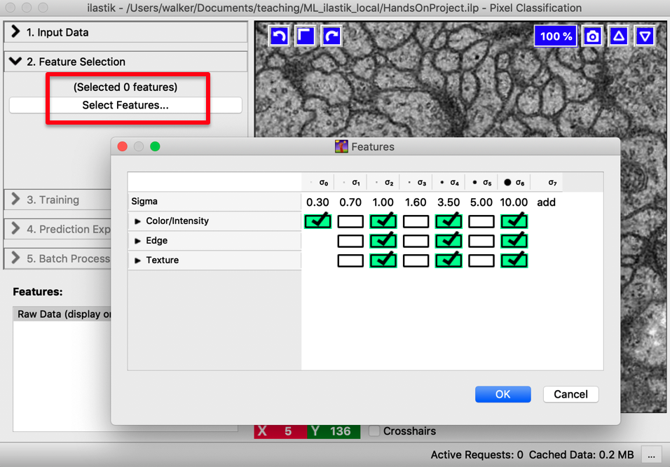 | (b)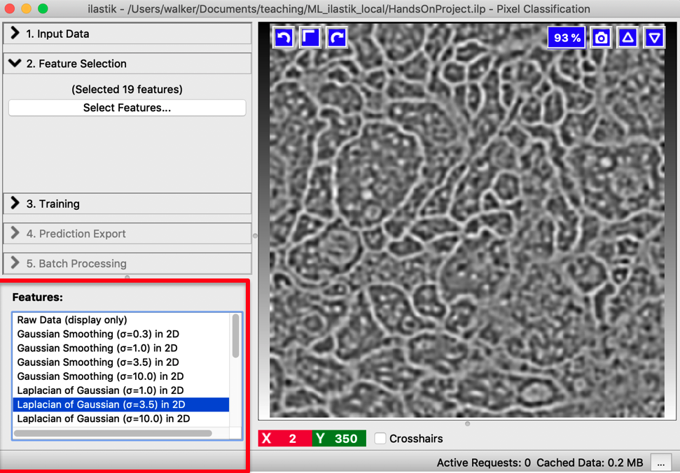 |
Step 4: Training
- Select Training tab.
- (a) Double-click on the colored Labels to give more descriptive names to your classes (e.g. cells and background). Optionally add more labels.
- (a) Use the brush tool to paint some regions for each class in the correct label color. This process is called “ground truth creation”.
Basic Navigation:
Mouse: Zoom: Cmd/Ctrl+wheel, Pan: Shift + left button
Keyboard: Zoom: +/-, Pan: arrows keys - (b) Start the training by pressing Live Update.
- The classifier trains based on your labelled regions and shows the predictions as overlay.
If needed, change brightness & contrast (blue arrow in (b), a right click resets the display range). Alternatively, right-click on the image in group visibility Tab > Adjust thresholds.
Group Visibility tab (see (b)): Switch between probability and segmentation overlay. Change overlay transparency with the slide.
(a)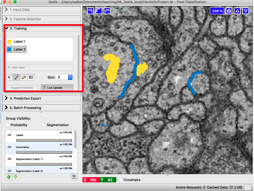 | (b)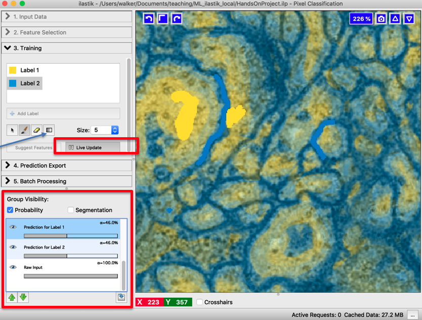 |
(c)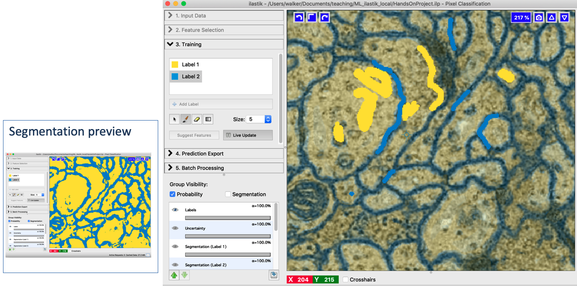 | |
- (c) If prediction is not good, paint more regions. This increases the number of training pixels.
- If preview is slow uncheck the Live Update while drawing.
- (c) Check the improved prediction after labelling more regions.
- Don’t forget to save your project regularly: Project > Save Project….
Step 5: Optional: Optimize training
- (a) If predictions are still not good, investigate your feature selection:
- Select Suggest Features (uncheck Live Update)
- Compare the predictions and choose the best feature set.
- (b) The uncertainty layer can also give you an indication which extra regions are good to label.
(a)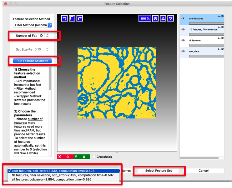 | (b)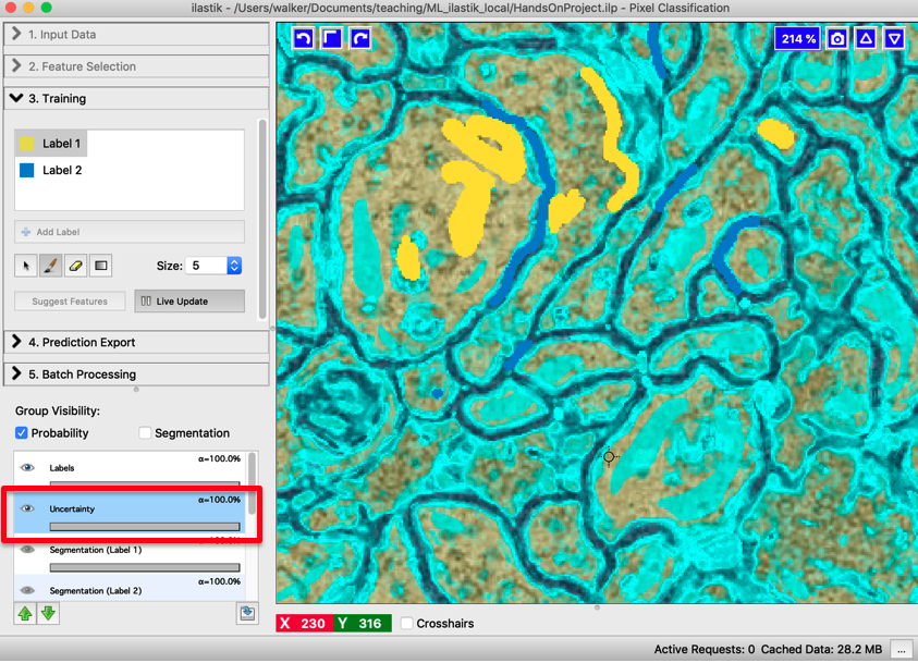 |
Step 6: Export predictions
Predictions can be exported as probabilities or simple segmentation. Exporting as probabilities is recommended as it provides more flexibility for downstream steps in tools like Fiji or python (for example: smoothing).
Export Probabilities
- Select Prediction Export tab.
- (a) Select Source: Probabilities, then press Choose export image settings.
- (b) Choose these settings:
- 2D image:
- Format: tif sequence
- If getting export error message: Select Transpose axis order: cyx
- 3D image:
- Format: multipage tif sequence
- If getting export error message: Select Transpose axis order: czyx
- File: optionally append the path with a /output/ subfolder
- Verify under Description that we get one image per label class (“c”).
- Then press OK to close the window.
- 2D image:
- (c) Press Export.
- (d) The created images can be opened in Fiji.
If the images seem black adjust the contrast to [0,1]: Image > Adjust > Brightness/Contrast
(a)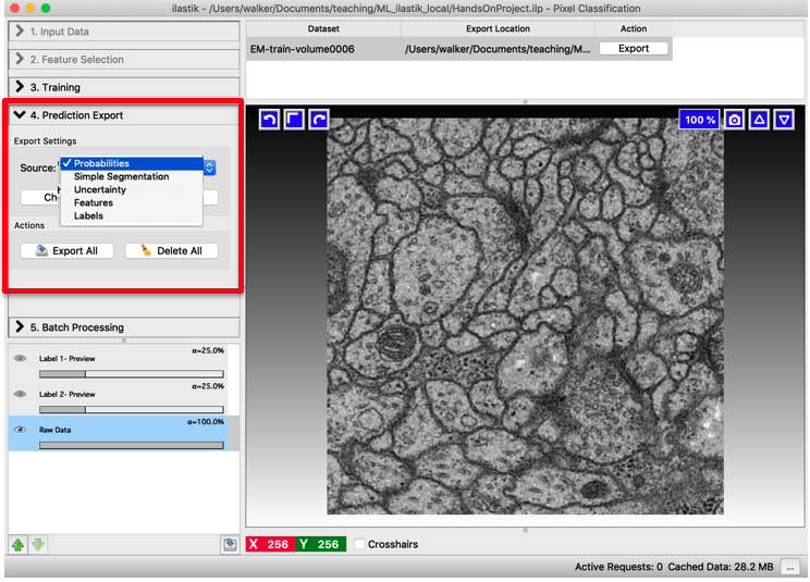 | (b)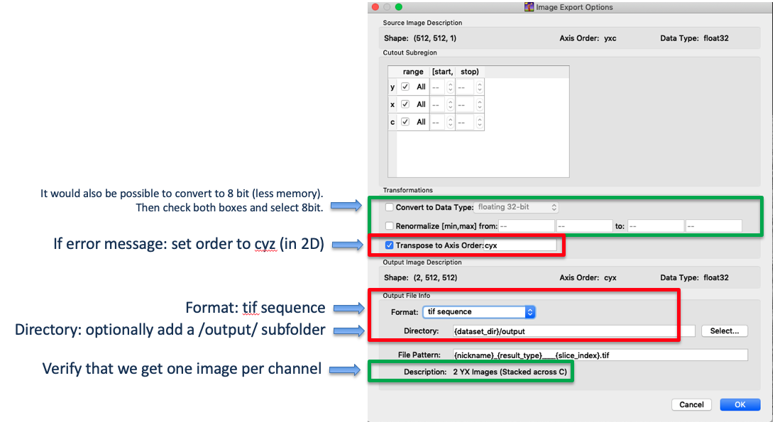 |
(c)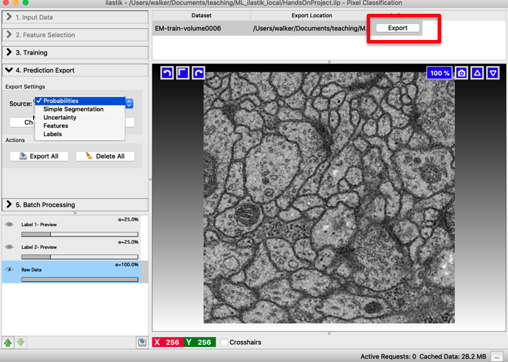 | (d)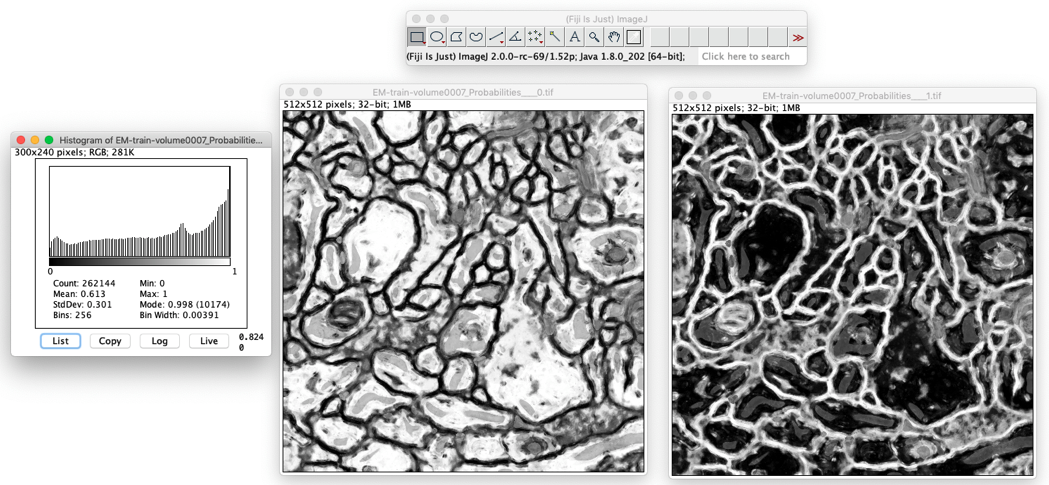 |
Export simple segmentation
If the segmentation is very simple, a direct segmentation export may be enough (and is easier):
- Select Prediction Export tab.
- Select Source: Simple Segmentation, then press Choose export image settings.
- (a) Choose these settings:
- Format: tif
- File: optionally append the path with a /output/ subfolder
- Then press OK to close the window.
- Press Export.
- (b) The created images can be opened in Fiji.
If the images seem black adjust the contrast to [0,2]: Image > Adjust > Brightness/Contrast
(a)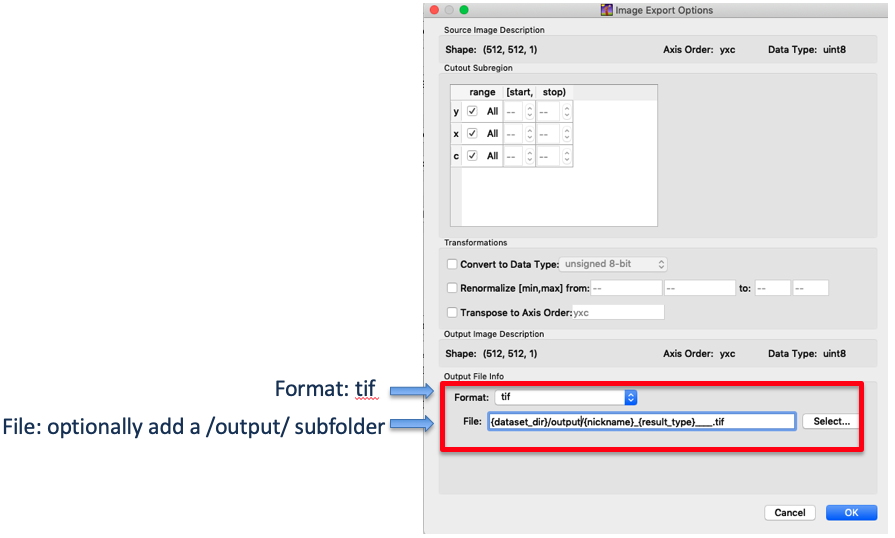 | (b)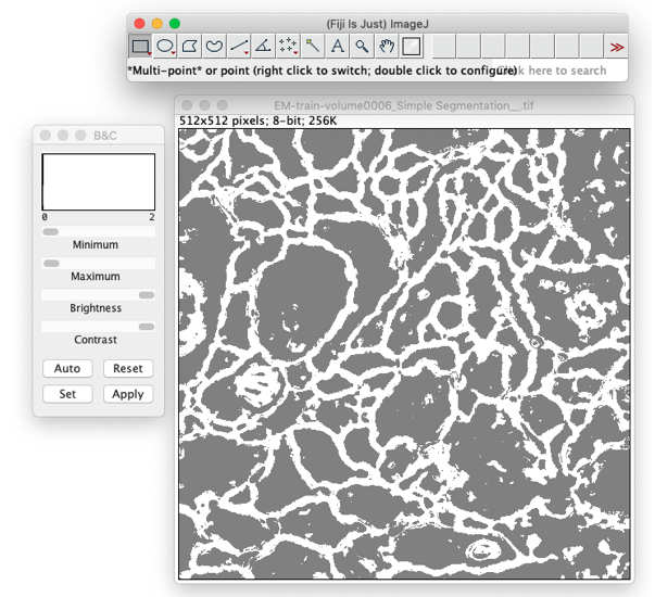 |
Step 7: Batch processing
- To make predictions for all your images (which were not used during training), select the Batch processing tab.
- (a) Click Select Raw Files… and browse for your images.
- (b) Press Process all files to start batch prediction.
(a)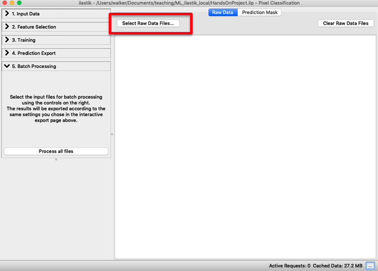 | (b)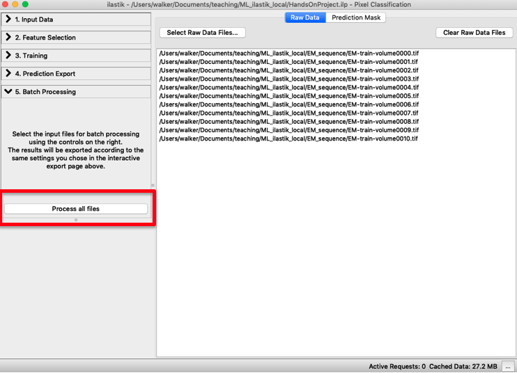 |
Tips & Tricks
- If images have high variability:
- Train on representative subset
- Standardize images beforehand (e.g. histogram equalization, normalize to robust min/max)
- If objects are touching it is helpful to introduce an “object border” class and assign a thin line around the object to this class.
- Importing results into Fiji: if error, use BioFormats importer.
- There are lots of options for post-processing the exported probability map in Fiji:
- Optionally initial smoothing
- Can set custom threshold value
- Can combine different classes (if >2 classes)
- Ilastik also has a Fiji plugin:
- Convert data to their favorite format (hdf5)
- Run Ilastik pipeline from Fiji.
Alternatives
Two Fiji plugins work with similar segmentation algorithms and labelling+prediction workflows as Ilastik: