Deconvolution using HuygensPro
Huygens
- Introduction
- Step-by-step
- 1. Data acquisition
- 2. Data transfer
- 3. Deconvolution using Huygens
- Comment: Experimental PSF
- Tips & Tricks
- Alternative Software
Introduction
Optical systems like microscopes produce images that are not perfect but degraded by blur and noise. Technically, the blur is the result of a convolution of the “ideal” image with the so-called point spread function.
The point spread function (PSF) is the 3D image produced by a point-like source. Its shape and size depend on the microscope type, wavelength, objective, refractive index of immersion and sample medium etc. The PSF can be measured experimentally with sub-resolution beads or be calculated.
Deconvolution is an image restoration process that recovers an image which was degraded by convolution. It inverts the convolution process. For more details on deconvolution also see the documentation from Huygens.
Deconvolution increases image quality and image resolution. It improves contrast and reduces noise and background signal. Using deconvolution is very important for colocalization analysis and precise shape measurements.
Huygens software
Huygens is a deconvolution software available at CBG. Additional capabilities include chromatic aberration correction and colocalization analysis.
Features of Huygens at CBG
- Currently, licenses are available for deconvolution of images acquired with confocal, spinning disk, widefield systems.
- Two versions of Huygens are available:
- HuygensPro: GUI-based, useful for exploration of new data
- Huygens Remote Manager: browser-based, useful for batch processing
- HuygensPro (the content of this how-to guide) is installed on a Linux server and can be accessed remotely from your laptop.
Requirements for accessing HuygensPro
- Internal CBG network: You need to be connected to the internal network. If working from a different network, connect via VPN.
- Login credentials: Contact IPF to obtain the login information to access HuygensPro.
This how-to guide is about a basic deconvolution pipeline using HuygensPro and a calculated point spread function.
Step-by-step
The step-by-step section is split into (1) data acquisition, (2) data transfer (3) deconvolution.
Important: Deconvolution is not a one-click-done process. Always inspect your results critically for quality and artifacts and redo the analysis with different parameters if needed.
1. Data acquisition
- Correct data acquisition is very important for good deconvolution.
- A general rule of thumb: give more importance to sampling than signal, i.e. noise is acceptable but not undersampling.
- If you plan to use measured PSF, make sure to acquire fluorescent bead images as well.
General guidelines
- High spatial sampling
- Make sure you sample your data well, especially in Z. Use the Nyquist calculator to get the ideal Nyquist sampling rate.
Confocal: up to 40% undersampling is acceptable as compared to the ideal sampling.
Widefield: stick to the ideal sampling rate as much as possible.
- Make sure you sample your data well, especially in Z. Use the Nyquist calculator to get the ideal Nyquist sampling rate.
- Accept noise
- high sampling is more important than avoiding noise.
LSM acquisition: for very low intensity: use accumulation or photon count instead of averaging.
- high sampling is more important than avoiding noise.
- Z-stack range
- image till the edge of the object + ½ PSF above and below sample. Especially important for Widefield.
- No saturation and clipping
- Avoid saturating your image, the image does not have to look pretty!
- Metadata
- Save the image in a format that keeps all the metadata.
- Use sufficiently high bit depth (typically 16-bit).
Deconvolution is not possible if:
- the volume is 2x undersampled, and/or
- image is heavily saturated or clipped.
Tip 1: Check the Huygens webpage for more details on proper image acquisition (ask IPF for login).
Tip 2: Talk to your microscopists before deconvolution, involve the image analysts as well.
2. Data transfer
- Your raw data has to be transferred to our Huygens computer for processing.
- This can be done by mounting the Huygens computer as project space:
- Mac users:
- Start Finder.
- In the menu bar click on Go and select Connect to Server…⌘K
- Type
smb://lmfuser@huygens-srv1.mpi-cbg.de/UserData - Click Connect.
- Windows users:
- Open the Explorer (not Internet Explorer).
- In the path bar type
\\lmfuser@huygens-srv1.mpi-cbg.de\UserData. - Press enter.
- Mac users:
- Enter the login credentials (obtained from IPF).
- Once connected, navigate to the folder named UsersDataFolders.
- Create a folder of your name.
- Copy only the data that needs to be processed to this folder.
- After performing deconvolution, make sure to transfer back the data to your local machine or project space.
Important: The data on Huygens computer is not backed up and will be cleared on a regular basis.
3. Deconvolution using Huygens
Prerequisite: Microsoft Remote Desktop application is required to connect to the Huygens computer.
On Windows, Remote Desktop Client / Connection is installed by default.
On Mac, you need to download and install MRD version 8 or 10 from here or the AppStore.
Step 0: Book Huygens using the booking database.
- The booking database can be reached with this link: LMF Booking System.
- Use your normal CBG credentials.
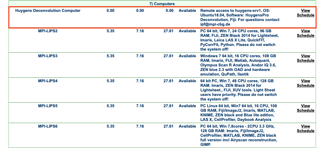
- The service is listed under Equipments Tab > Computers > Huygens Deconvolution Computer.
- Booking is essential!
Step 1: Connect to Huygens Computer
- Open Microsoft Remote Desktop.
- (a) Select the PCs tab and click on the Add PC button on the main window. Alternatively, one can also click on the ‘+’ button on the top menu bar and select Add PC.
- (b) Enter the details.
- PC Name: huygens-srv1.mpi-cbg.de
- User account: In the drop-down menu, select Add User Account and enter relevant credentials (obtained from IPF).
- Click on Add button at the bottom right.
(a)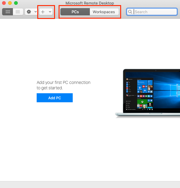 | (b)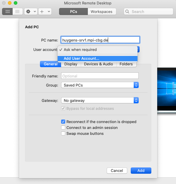 |
- You will see a computer added to the main window.
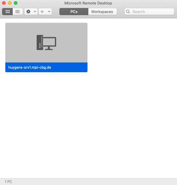
- Double click on the added PC to launch the remote desktop. If everything went well, you will have a desktop window like below.
Step 2: Launch HuygensPro
- Launch Huygens by double-clicking on the Huygens Professional icon on the remote desktop.
- The main window has the following appearance.
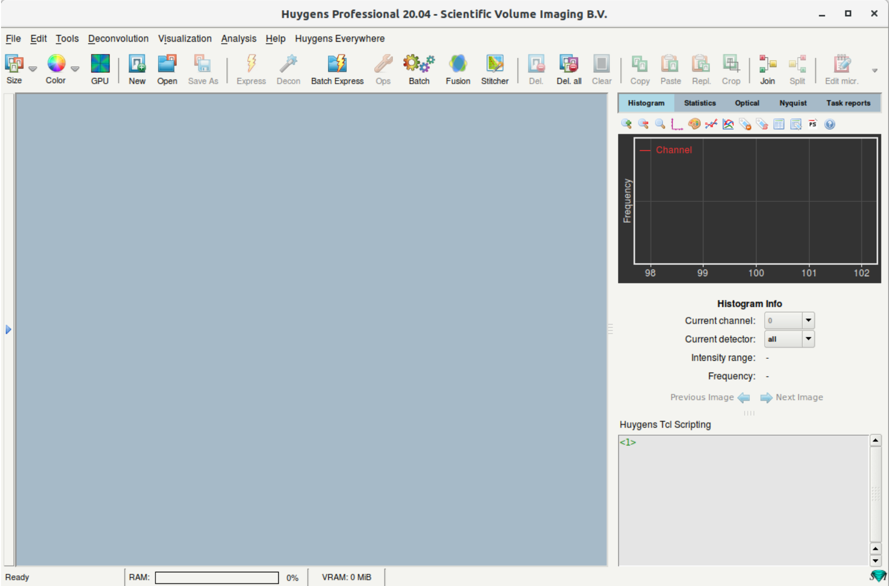
- Main sections:
- The blue region is where you will find the thumbnails of opened images and processed results.
- On the top is a taskbar with icons to launch main functions such as deconvolution (Decon) and batch processing (Batch Express).
- On the right, the window with multiple tabs gives you information related to the currently selected image.
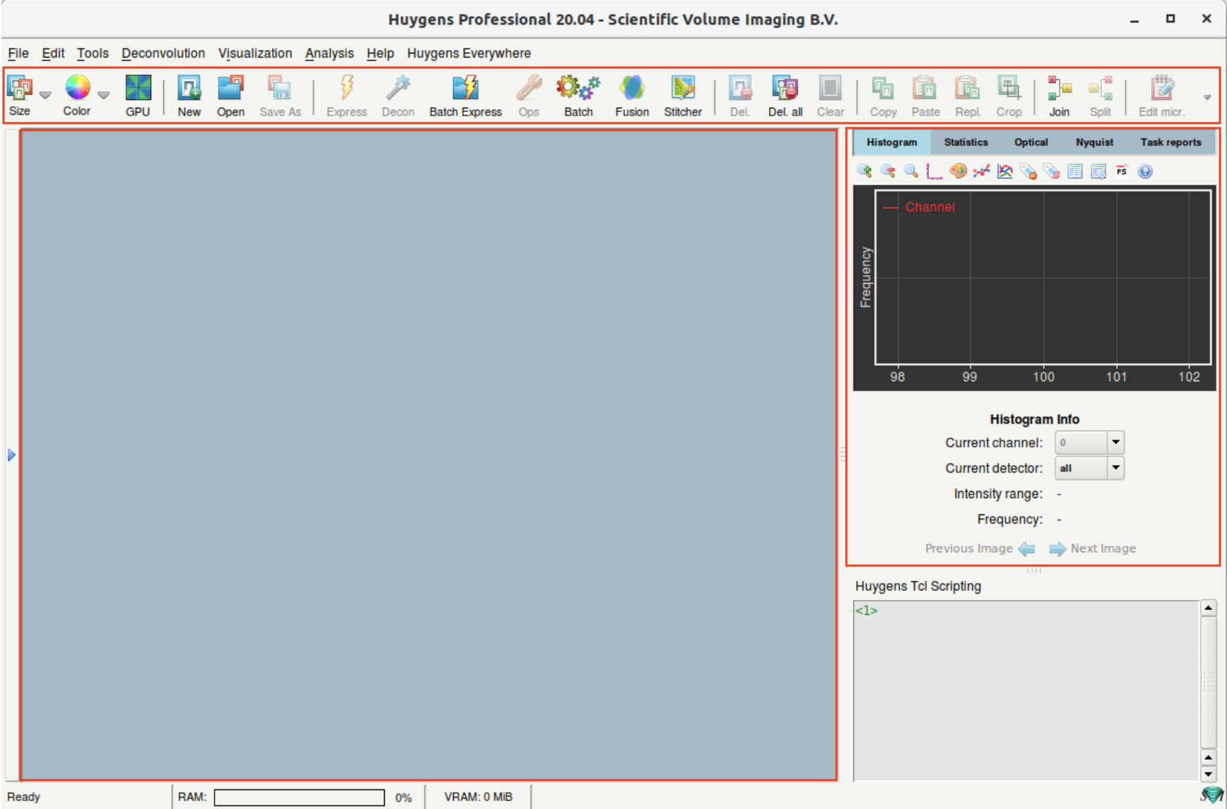
Step 3: Open an image file
- (a) Click on the Open button to open an image. Alternative: File > Open
- (b) On opening an LSM image, Huygens will ask for the microscope model used for imaging. Select the one you used for image acquisition; contact the LMF if you are not sure.
- (c) On opening a TIF series, Huygens will ask how to interpret the individual files. Such as slices from a 3D stack, channels or time points.
(a) | (b) |
(c)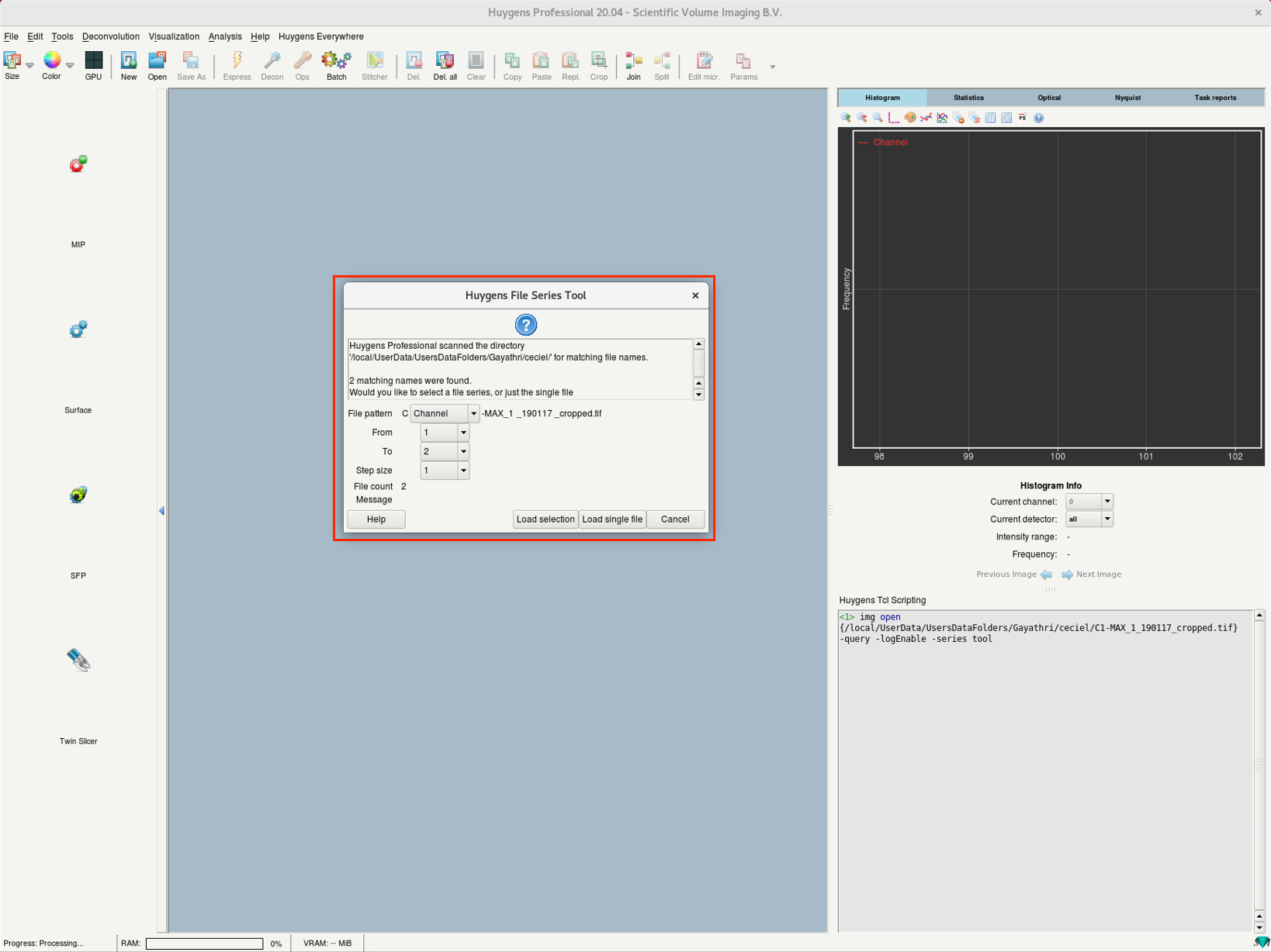 |
Step 4: Inspect your image
- After opening a file, you should find a new image thumbnail in the main workspace.
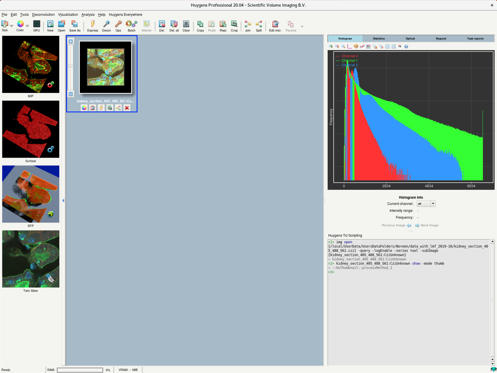
- Click on the thumbnail to select the image.
- Once you select:
- the right window is updated with the image histogram and other information, and
- the windows on the left show multiple renderings of the selected image.
- Right-click on the thumbnail and select 2D Visualization > Slicer. Alternative: Visualization > Slicer
- The Slicer view which allows you to check if the data was imported properly.
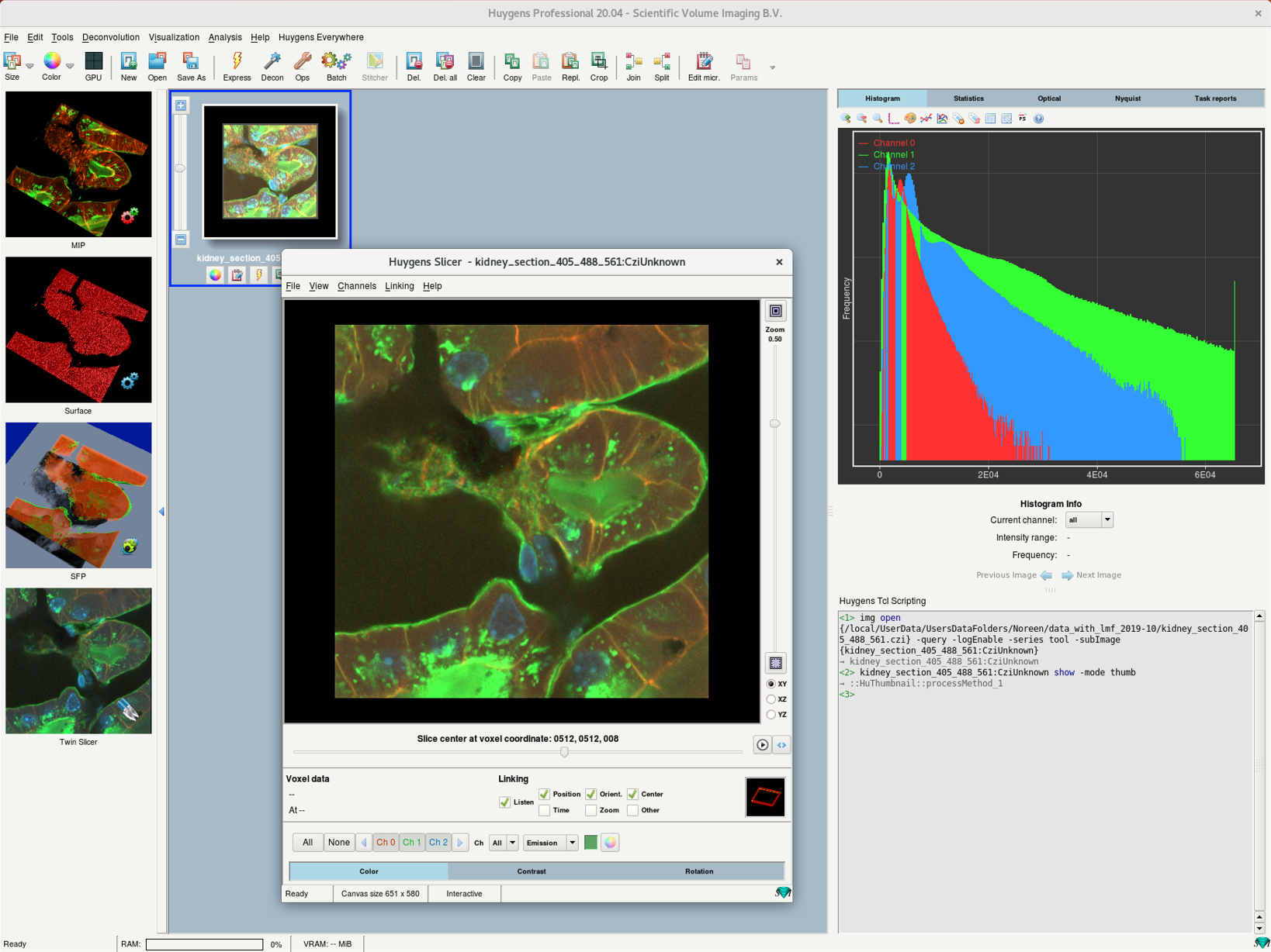
- There are controls to select any plane orientation in space (XY, YZ, XZ), zoom, scroll through slices, and view time frames (if applicable).
- Check if the image shows misalignment across the channels in case of multichannel image (chromatic aberration) or drift in Z for 3D time series.
Chromatic aberration can be corrected in Huygens using the menu Deconvolution > Chromatic Aberration Corrector.
The z-drift corrector tool is available as a part of deconvolution post-process for 3D time-series.
Tip: If the image dimensions are not loaded correctly (for example, channels are read as slices) use the option Tools > Convert to set the right dimensions.
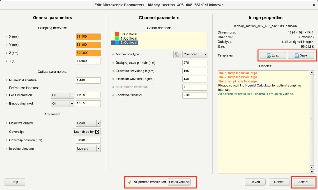
Step 5: Microscopy parameters
- For a good deconvolution result, it is extremely important to have accurate microscopic parameters since these values are used to compute the PSF.
- Right-click on the image thumbnail and select Microscopic parameters. Alternative: Edit > Edit Microscopic Parameters
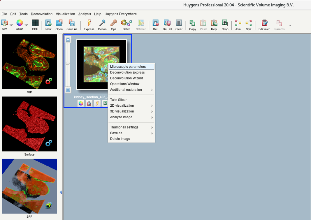
- Parameters are read from the image metadata.
- Sometimes, the values from the metadata are not read out correctly. Check and correct the parameters.
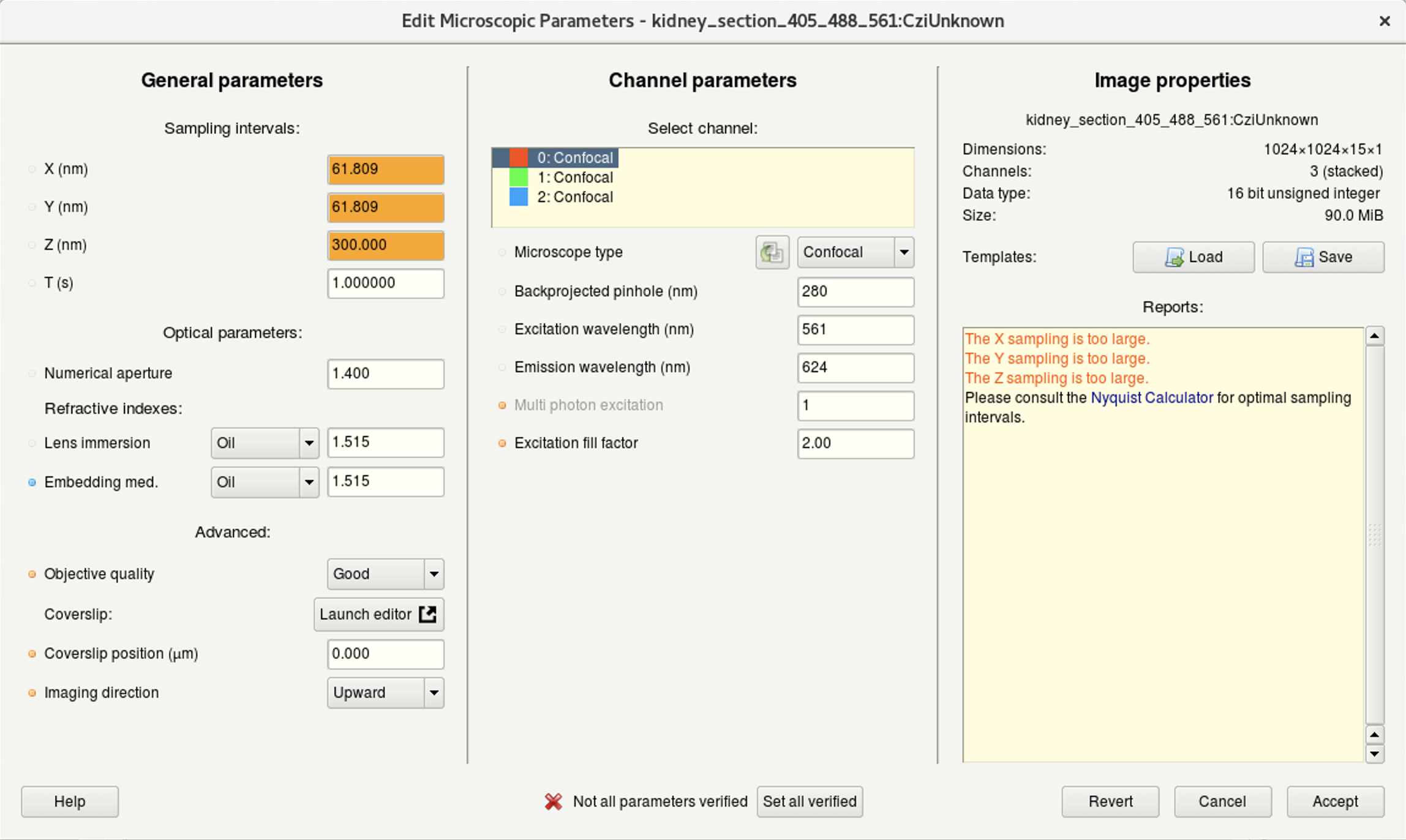
- Sub-windows (image below):
- (a) Here you can edit the general imaging parameters.
- (b) Here you can specify the microscope type as well as the excitation and emission wavelength for each acquired channel.
For a bandpass emission filter, you can use the center wavelength.
Multiphoton images: select Widefield and set the Multiphoton excitation to 2.
For standard microscopes, the Excitation fill-factor = 2 or higher.
For confocal microscope data, the Backprojected pinhole (nm) should be calculated correctly from the metadata (but double-check!).
- (c) Here you can find the summary of your image data.
(a)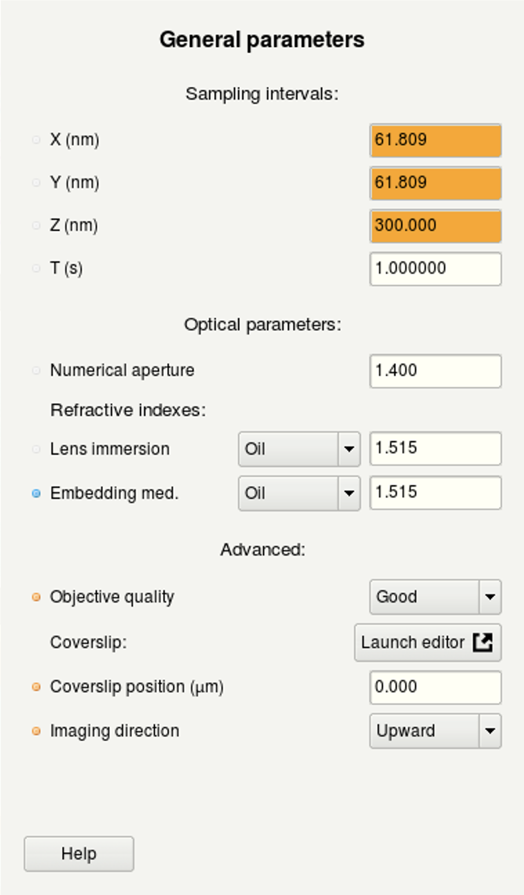 | (b)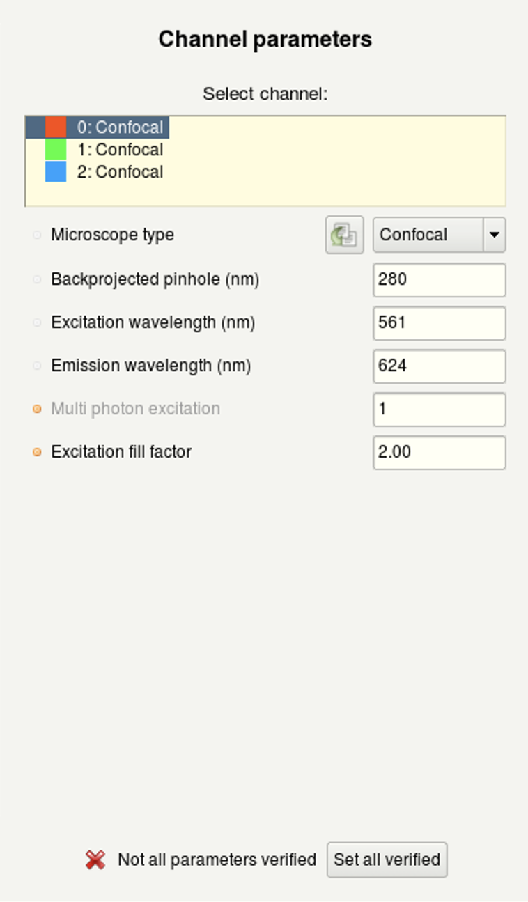 |
(c)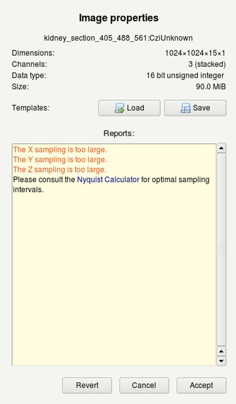 |
- Once you have correctly set and verified the parameters, click on Set all verified followed by Accept.
If you acquired multiple datasets with the same parameters, save them as a template for future use or batch processing.
The Load button serves to load a previously saved parameters template.
Tip 1: For more information on the Huygens microscopic parameters click here.
Tip 2: Huygens uses different background colors and the Reports window, to give you feedback about issues with your imaging settings or parameters.
Step 6: Deconvolution wizard
- Right-click on the image and select Deconvolution Wizard. Alternative: Deconvolution > Deconvolution Wizard or Decon icon on the task bar.
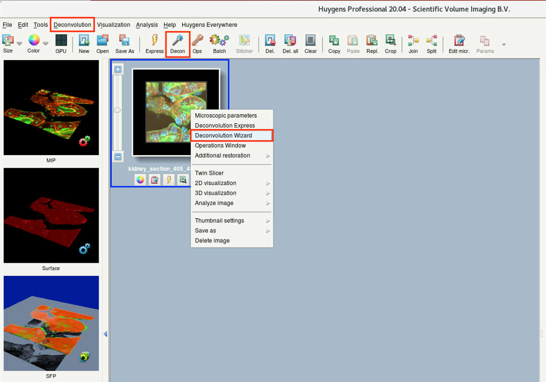
- On the start window of the wizard, you can see a summary of the previously defined parameters.
- The Wizard status window shows the current status, warnings, etc.
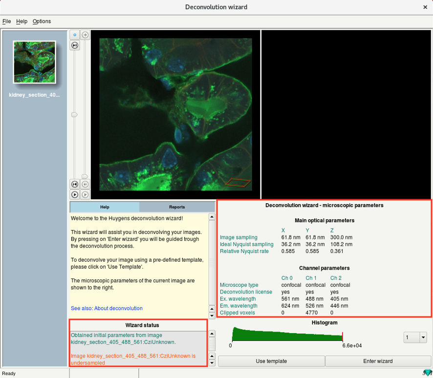
- Check if the parameters are correct and click on Enter wizard.
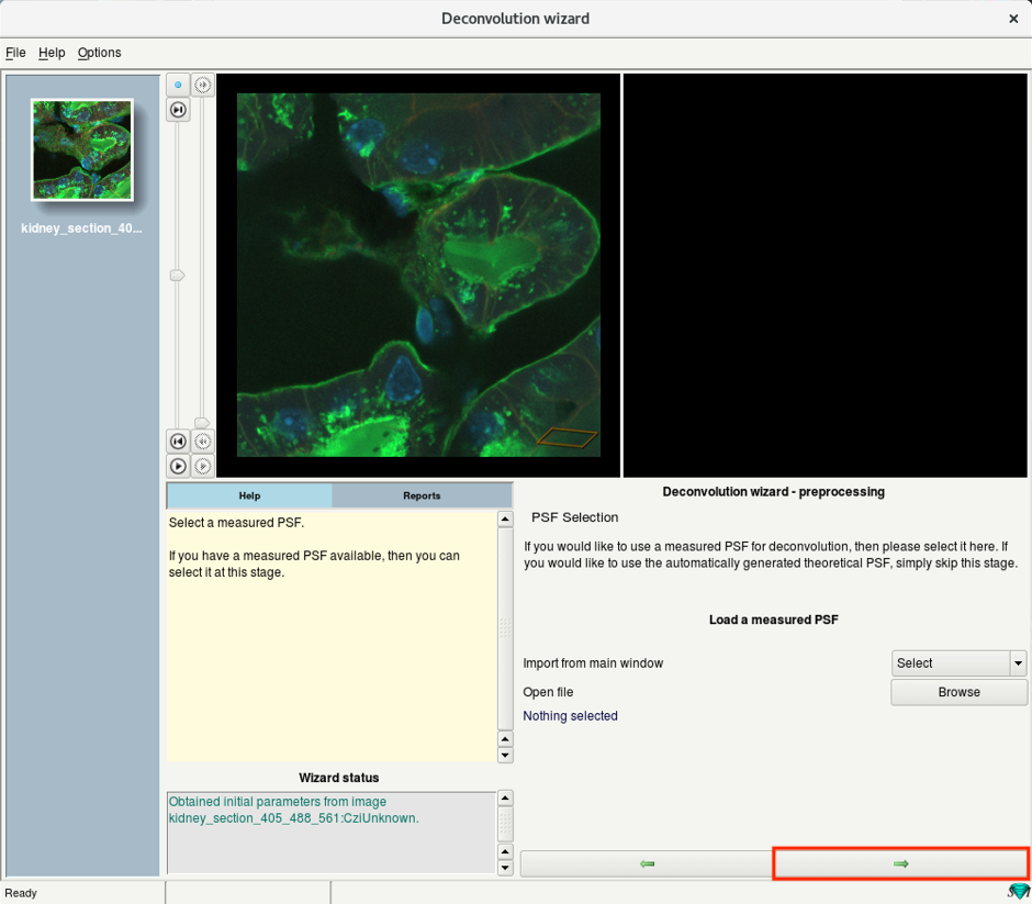
Step 6a: Deconvolution wizard: PSF selection
- Huygens supports both measured and theoretical PSF.
For thick samples, it is recommended to use theoretical PSF.
For badly aligned microscopes, better to use measured PSF.
- This how-to-guide uses a calculated PSF. If you want to use a measured PSF it needs to be acquired and prepared before launching the deconvolution wizard. See the section at the end of this page for a summary.
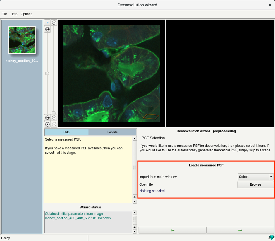
- To let Huygens calculate the PSF from your image parameters (theoretical PSF), simply press Next (—>).
Calculated PSF works well and is recommended.
Step 6b: Deconvolution wizard: Cropping
- Crop the 3D stack manually by using the Launch the Cropper option.
The time needed to deconvolve an image increases proportionally with its volume.
Cropping helps to accelerate the process.
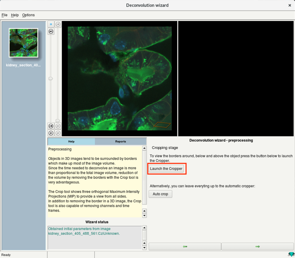
- Alternatively, one can also use the Auto crop to let Huygens automatically detect a suitable region of interest.
- If you launched the Cropper, set the region of interest by adjusting the boundaries of the bounding box.
- Press on Crop on the bottom right of the window.
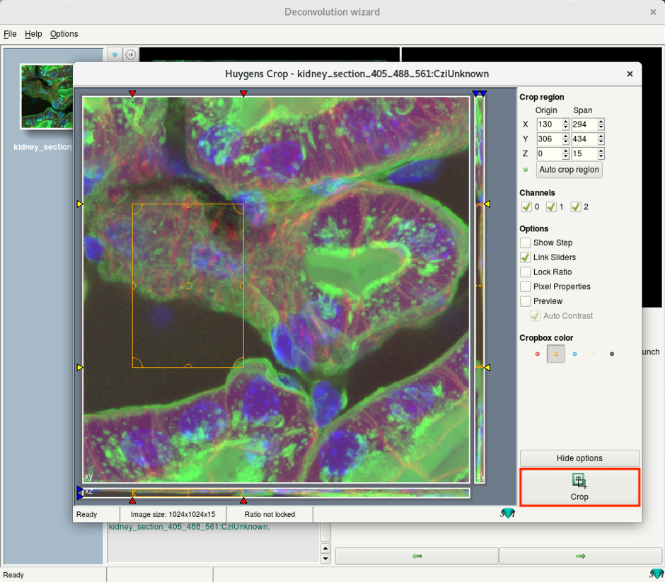
- Press Next.
Step 6c: Deconvolution wizard: Select channel
- If you have more than one channel in your dataset, you will need to deconvolve them sequentially.
- On the left, you will see all the channels of your dataset.
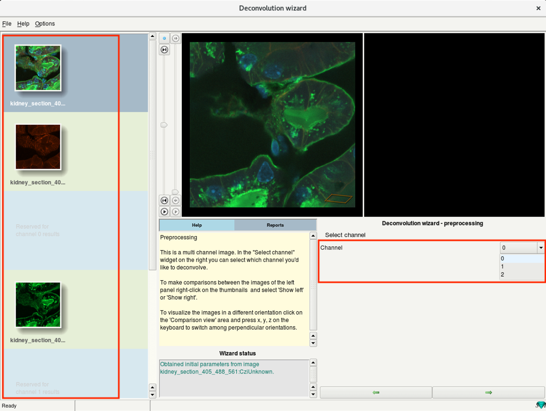
- Select the first channel from the drop-down menu on the right and press Next.
Step 6d: Deconvolution wizard: Inspecting the image histogram
- In this step, you will calculate and inspect the image intensity histogram of the selected channel.
- Select Logarithmic and click Compute.
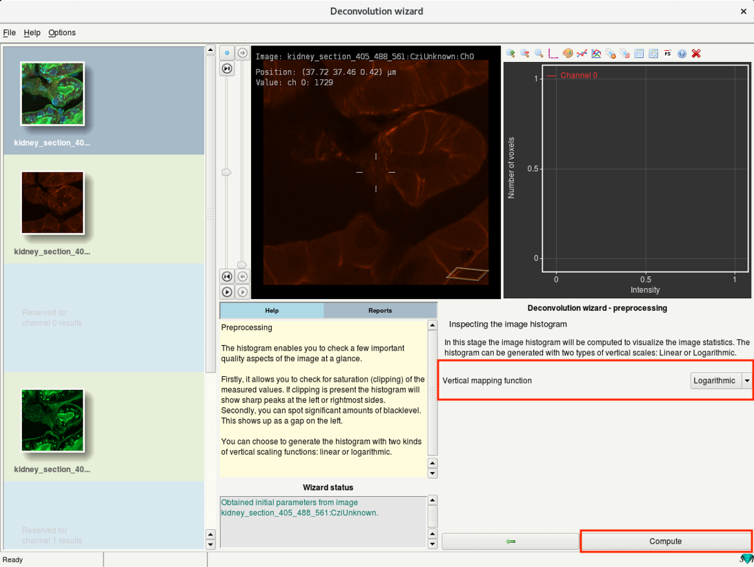
- Huygens computes the histogram and displays it on the window next to the image.
- Huygens also provides important information on the intensity distribution.
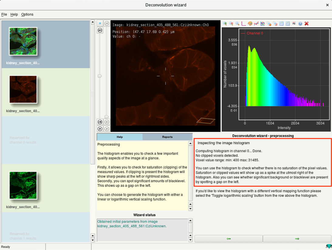
- Inspect the histogram and the report before proceeding.
A tall peak on the extreme right of the histogram indicates clipping or saturation.
Clipping occurs when input signals that are too high and are mapped to the highest possible value
A tall peak on the very left of the histogram also indicates clipping, here the negative input signals are mapped to zero.
There can also be an offset at the left of the histogram indicating a positive black-level. This does not affect the deconvolution results.
Tip 1: Save images as 16-bit to avoid clipping.
Tip 2: Avoid deconvolution if there are large regions of saturated pixels. Check and make changes to your image acquisition settings.
Step 6e: Deconvolution wizard: Background estimation
- Estimate the background intensity of the channel.
- There are two modes: Automatic estimation and Manual mode.
- It is recommended to use Automatic estimation.
Confocal: set Estimation mode to ‘Lowest’
Widefield: set Estimation mode to ‘In/Near Object’
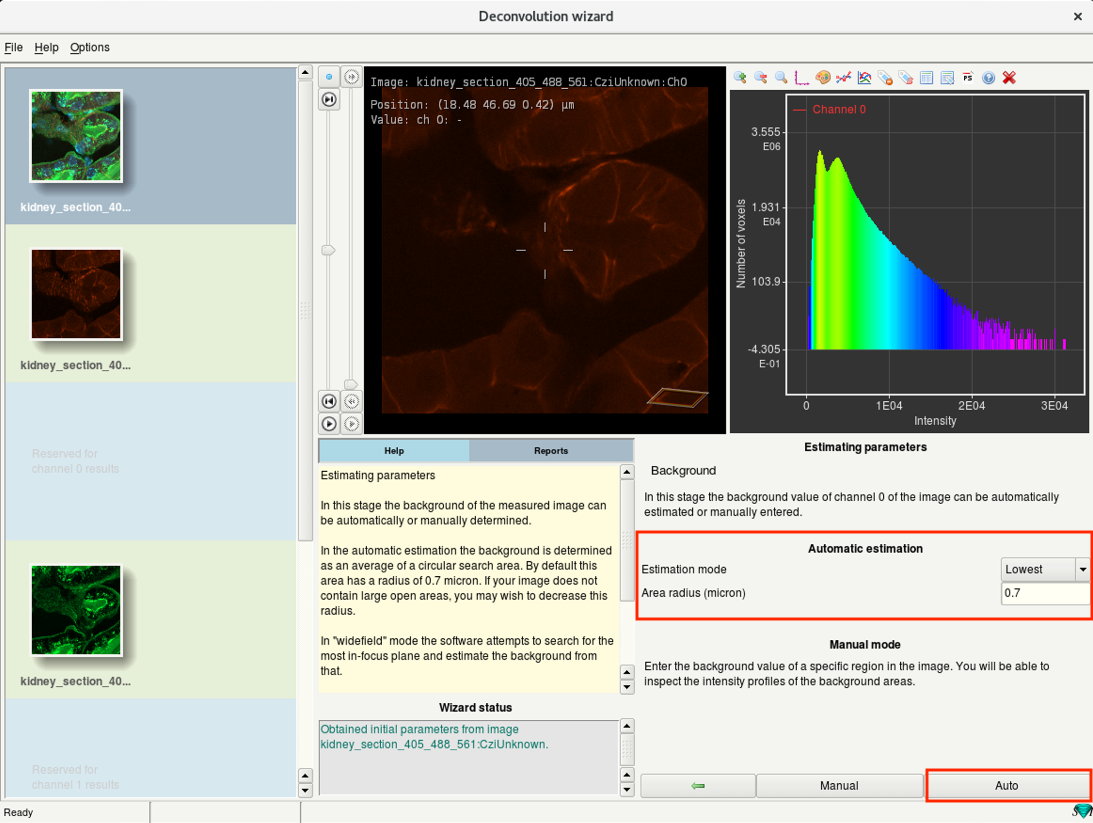
- Set the Estimation mode and click on Auto.
- To provide a background value with manual measurement, click on Manual.
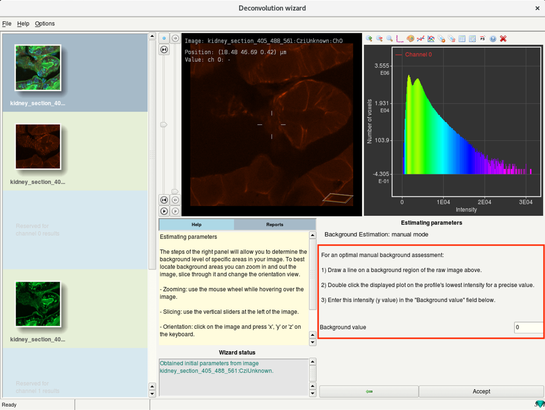
- Follow the instructions mentioned, enter the measured value in the Background value and click on Accept.
Step 6f: Deconvolution wizard: Select deconvolution algorithm
- If the Auto mode for background estimation was used, you will find the results here.
- Select the Deconvolution algorithm to be used.
CMLE(Classic Maximum Likelihood Estimation): Robust, default method.
GMLE(Good’s roughness Maximum Likelihood Estimaion): Good for high-noise images. Uses more memory than CMLE
QMLE(Quick Maximum Likelihood Estimation): Fast, good for low-noise images.
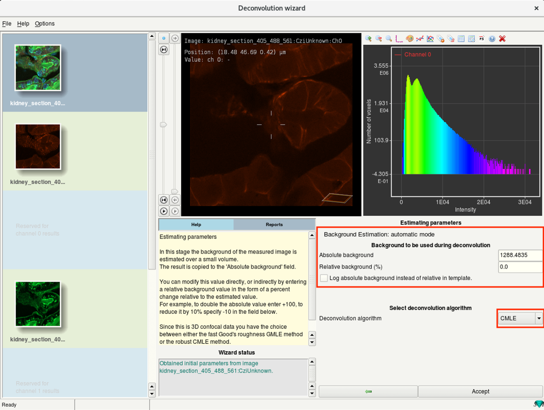
- Check the background estimate, select the deconvolution algorithm and click Accept.
Tip: CMLE is generally recommended for almost all kinds of images.
Step 6g: Deconvolution wizard: Setup deconvolution parameters
- The most important parameter that controls the deconvolution results is the Signal-to-Noise Ratio (SNR.)
- The SNR determines the sharpness of the restoration result.
SNR too low: harmless but no sharpening
SNR too high: causes artifacts
Noise-free widefield image: SNR approx. > 50
Noisy confocal image: SNR approx. 15-20
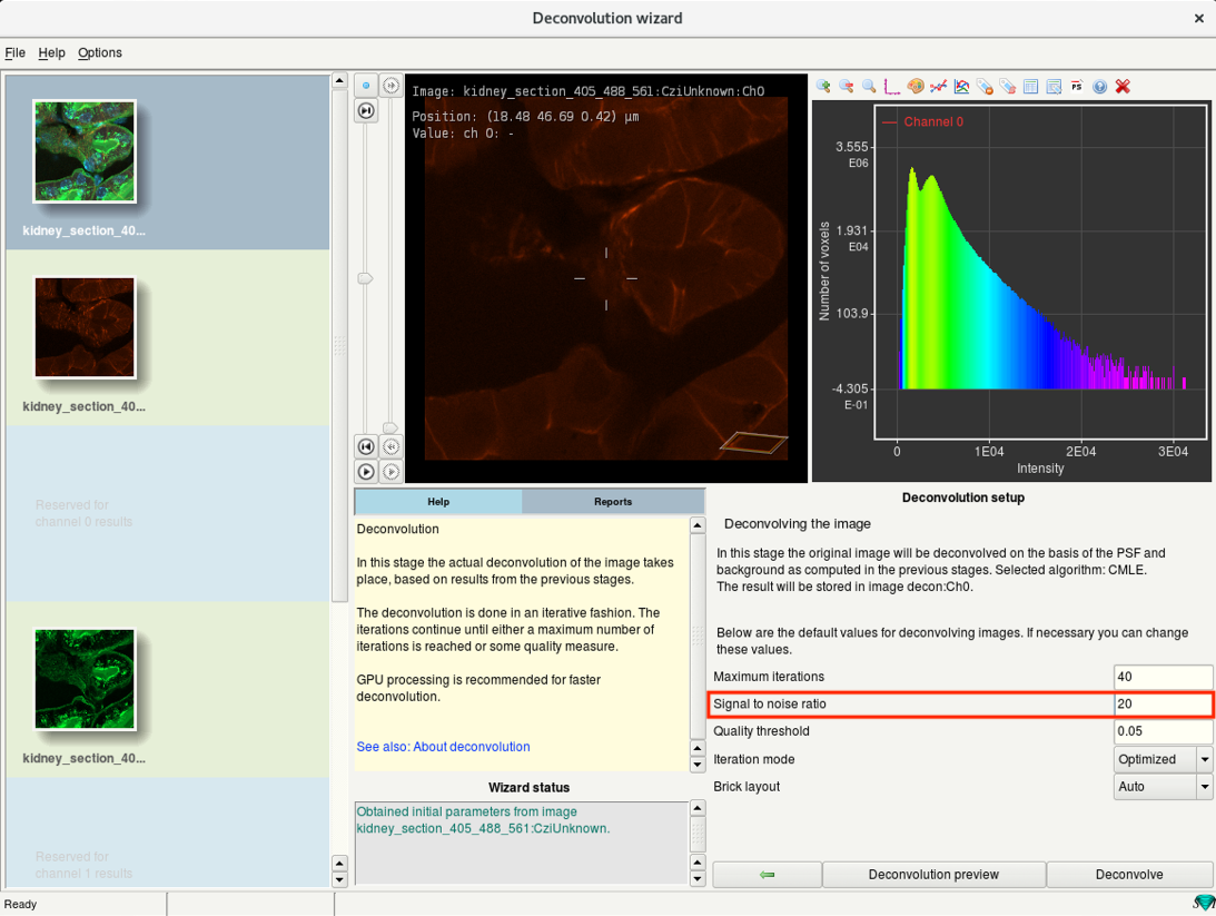
- Adjust the SNR value.
- For the others, the defaults are set according to the image parameters and require no adjustments.
Tip: Check the Huygens page for more details.
Step 6h: Deconvolution wizard: Preview and deconvolution
- Use the Deconvolution preview to check the results of current deconvolution parameters.
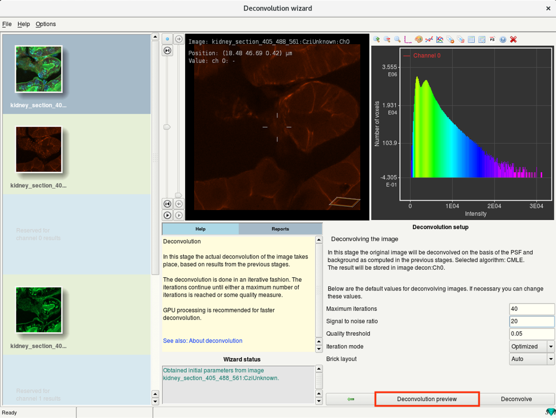
- The progress is visible in the Reports window on the left.
- In the image window, you can now see a yellow box which previews the result of deconvolution.
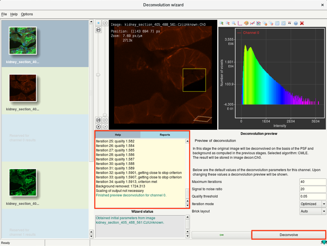
- You can move the box around to check the deconvolution preview from different regions.
Check for artifacts. If seen, reduce the SNR and test the preview again.
If there is hardly any change in the contrast, increase the SNR and run the preview.
- If the preview looks good, click Deconvolve. This will start the deconvolution of the active channel.
Tip: The SNR should be seen as a tunable parameter. The default is microscope-specific and a good start. But try different SNRs (10, 20, 40, 50), check the results and select the SNR which improves sharpness without enhancing noise.
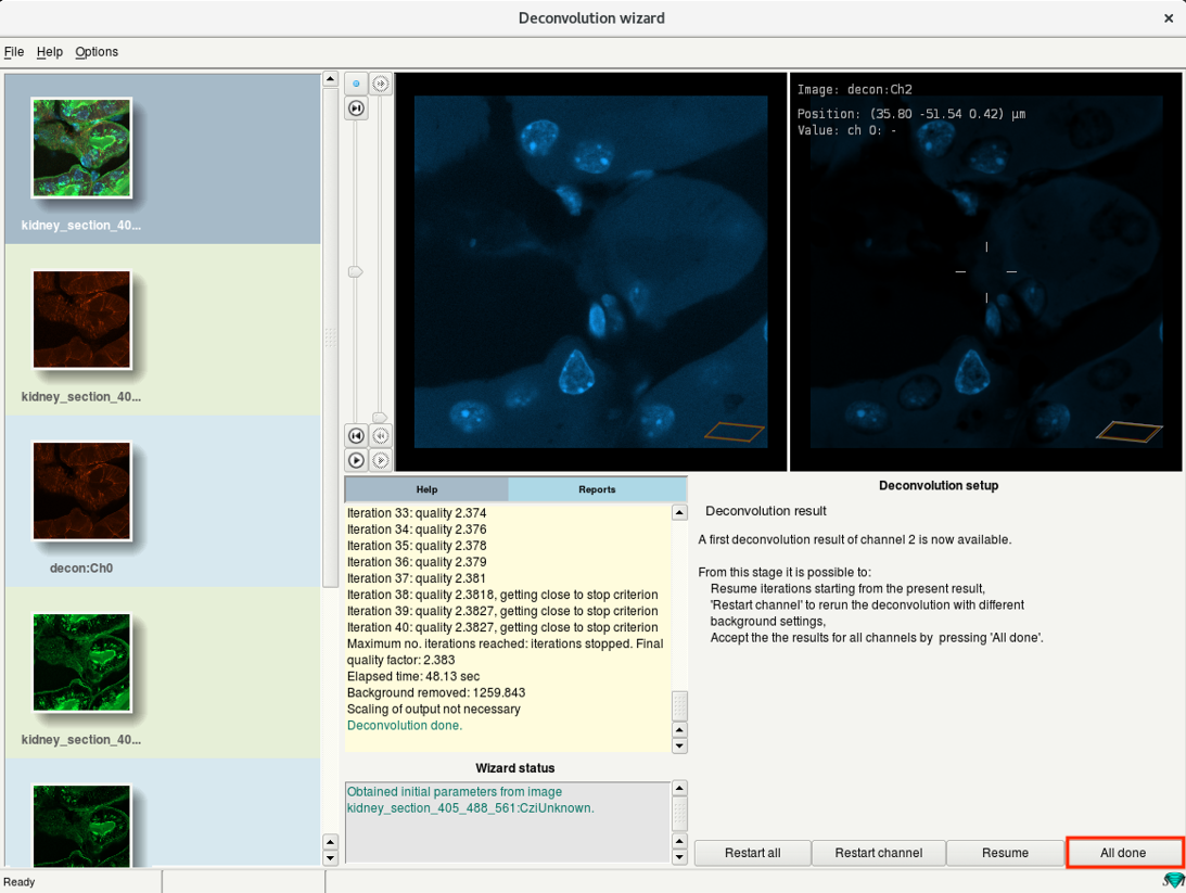
Step 6i: Deconvolution wizard: Deconvolution result
- When the deconvolution of your channel is done, you can see a preview of the result in the Deconvolution result step.
- Click Accept, to next channel to deconvolve the next channel of your dataset.
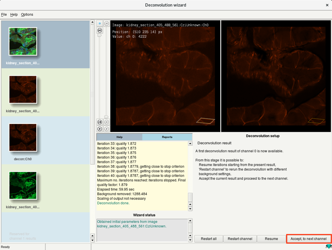
- For the next channel, the wizard starts at Step 6c.
- Perform a deconvolution for all channels of your dataset.
- After deconvolution of the last channel click All done.
Step 6j: Deconvolution wizard: Select the results
- You can merge the deconvolved channels here.
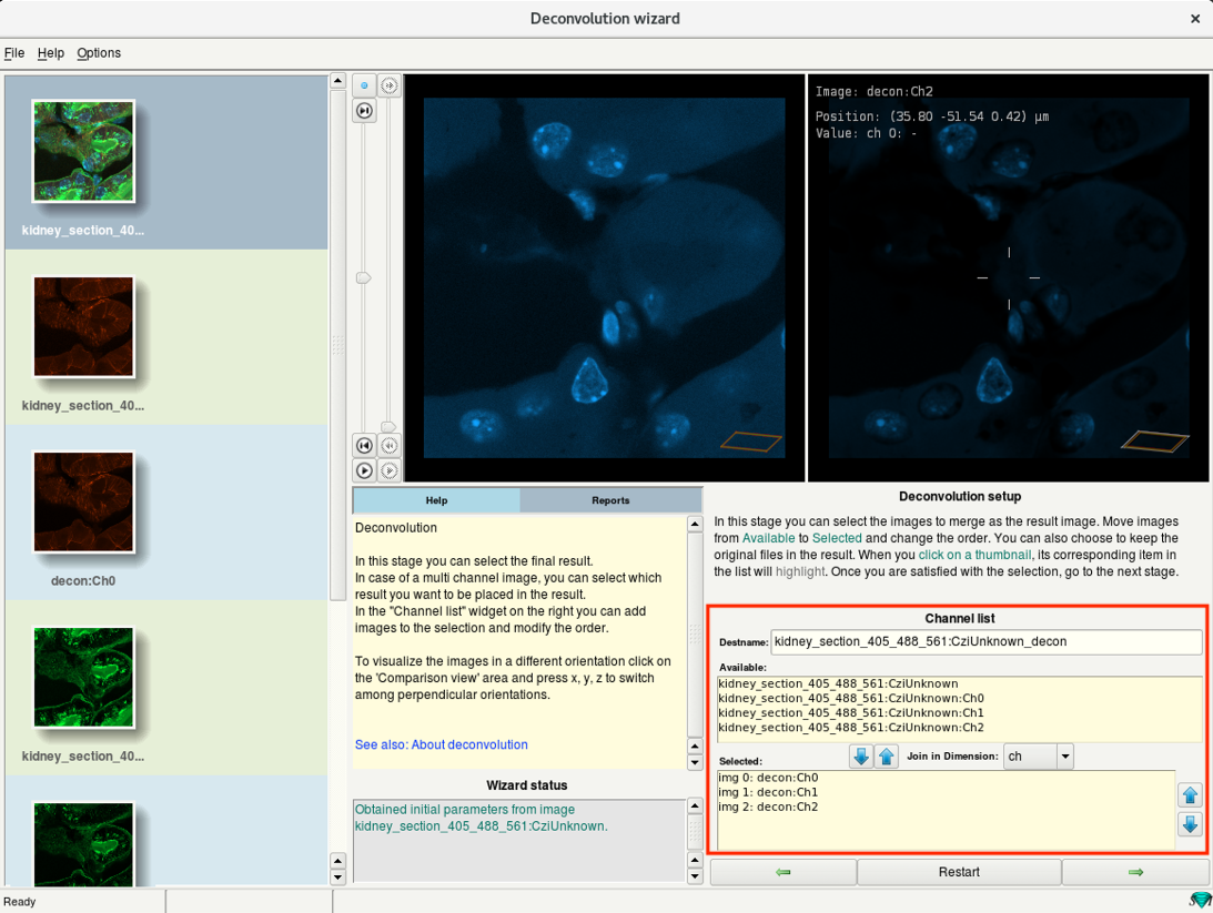
- Leave at default and click Next.
Step 6k: Deconvolution wizard: Summary
- In the last step you can save your deconvolution parameters as a template.
Useful if you plan to deconvolve multiple datasets of the same type.
- Click Done to close the deconvolution wizard and return to the main window.
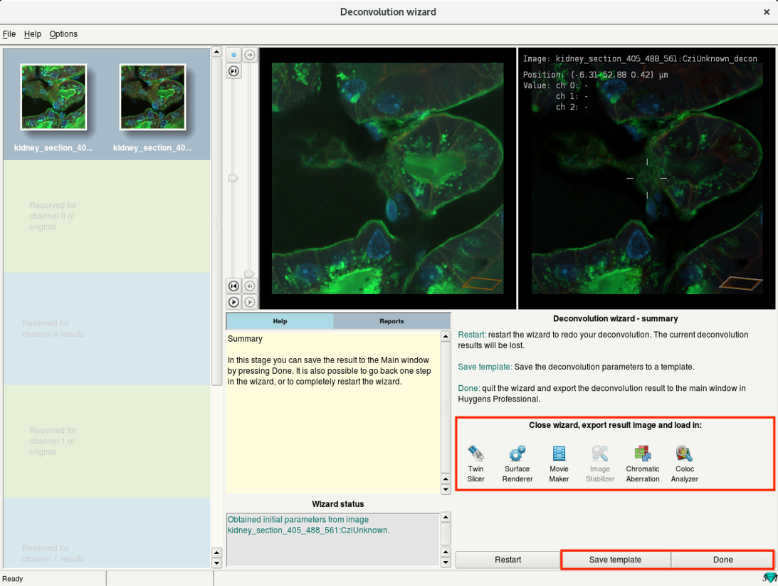
- Alternatively, click on Twin Slicer icon to close the wizard and export the results directly for exploration.
One can also go to other the postprocessing steps such as Chromatic Aberration correction by clicking relevant icons.
Step 6l: Explore your results
- If you clicked Done in the previous step, you will return to the main window where you will see a new image thumbnail of the deconvolution result.
- Right-click on the thumbnail and select Twin Slicer.
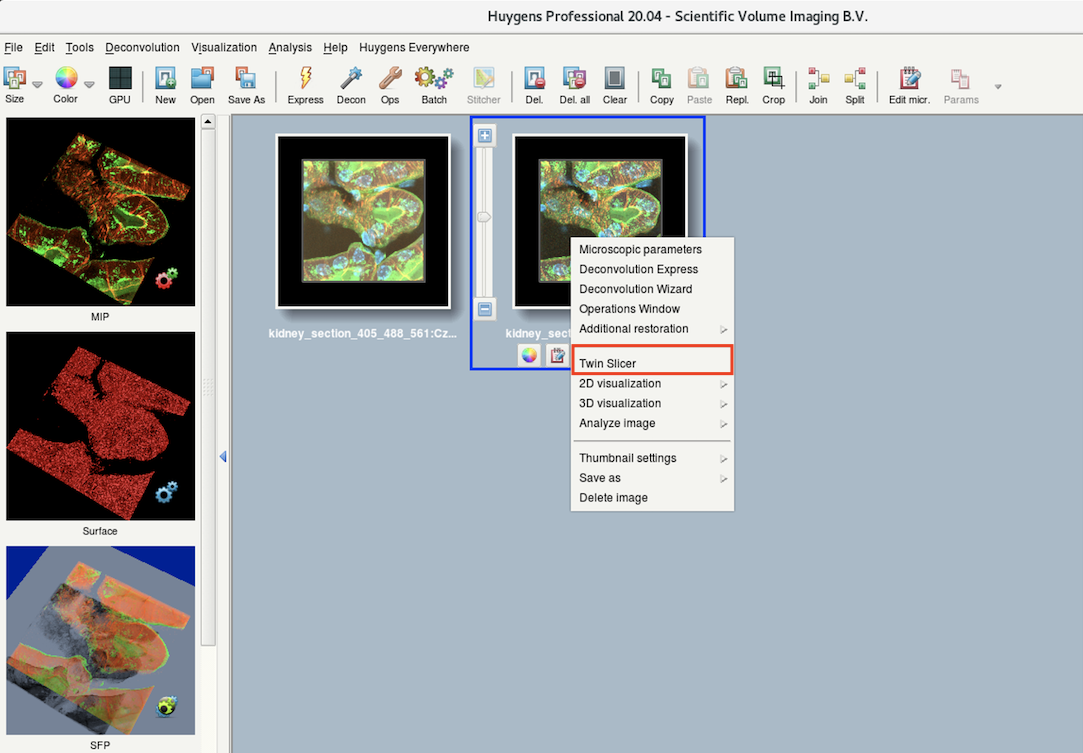
- Use the drop-down menu to select your raw dataset on the left and deconvolved dataset on the right.
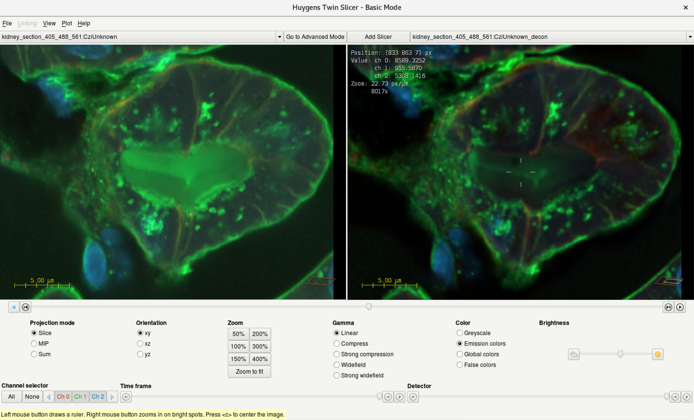
- Compare the deconvolution result with the raw dataset.
Step 6m: Saving your results
- Do not forget to save images before closing Huygens.
- Right-click the result image thumbnail and select Save As.
Recommended file-formats for saving: ICS2, TIFF 16-bit.
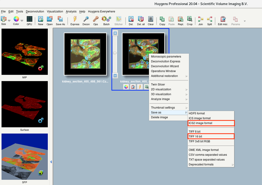
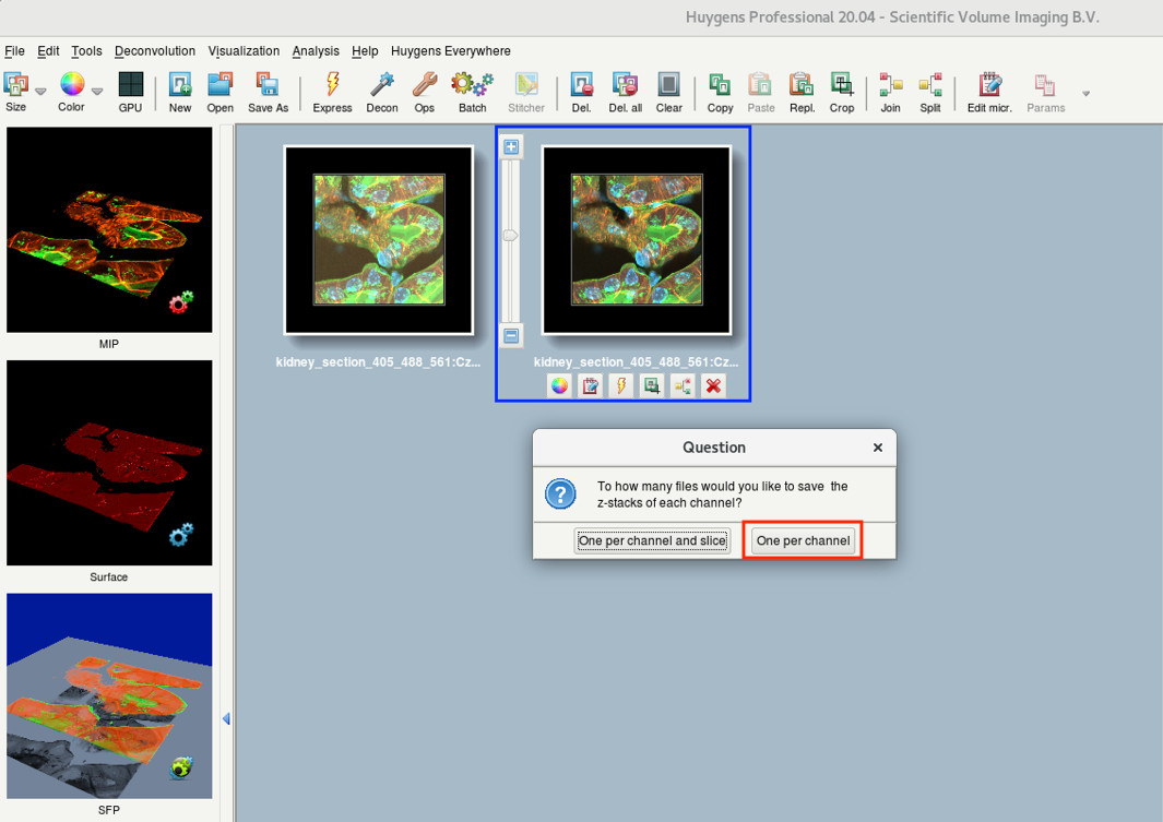
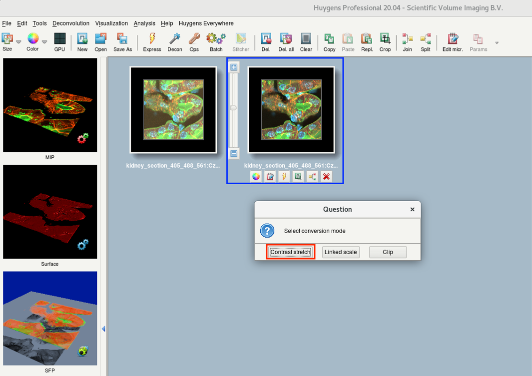
- A Question dialog asks you how you want to save your files. Usually One per channel is sufficient.
- Depending on the chosen file format and the intensities in your data, Huygens might also ask about the conversion mode.
Contrast stretch: good for visualization purposes and further analysis such as colocalization
Linked scale: use if you plan to perform ratiometric analysis.
Tip: Check the Huygens webpage for more details on saving images as TIFF.
Step 7: Quit Huygens
- Quit Huygens after usage by File > Quit.
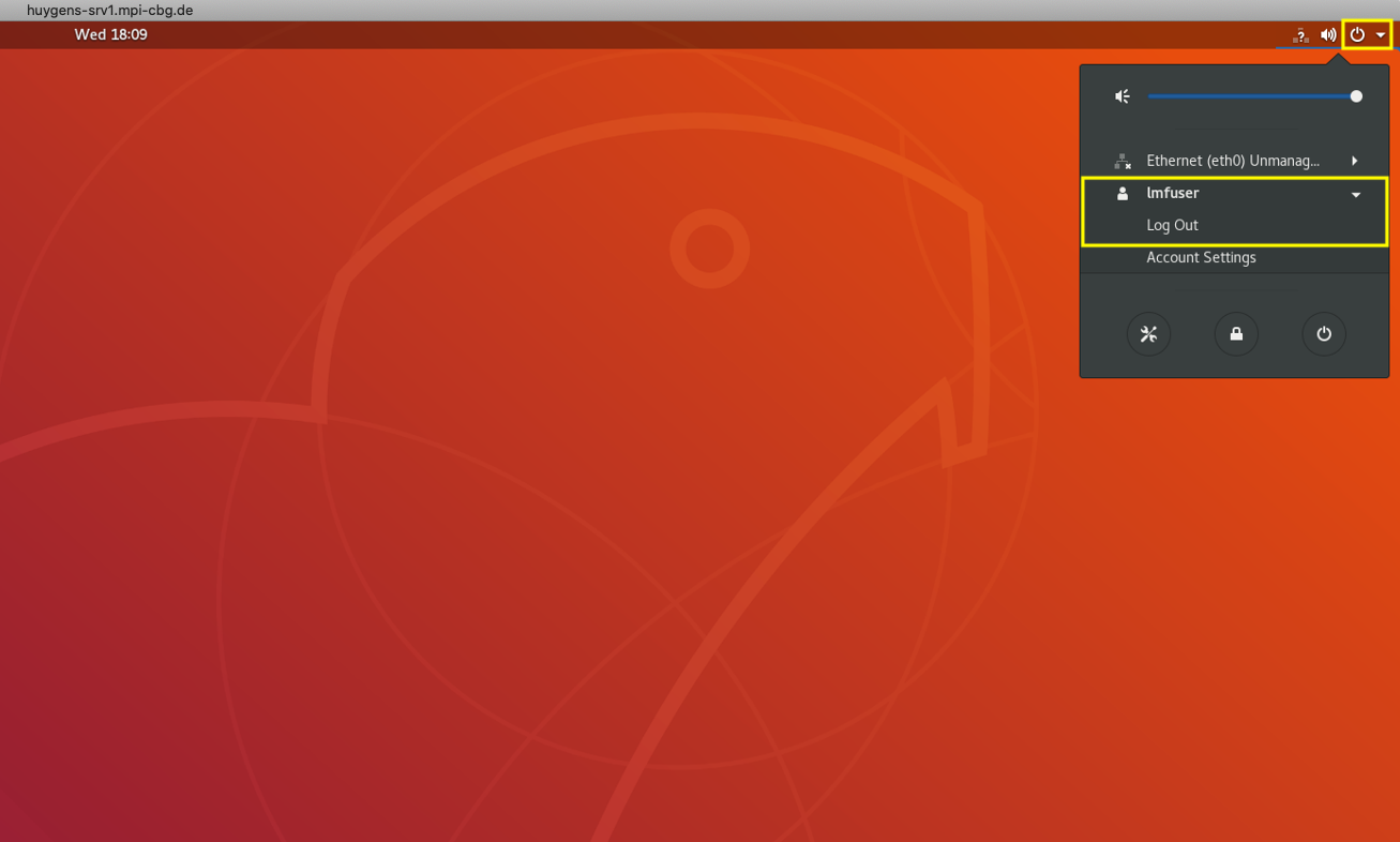
Step 8: Logout
- Once you quit Huygens, you will return to the desktop of the remote machine.
- Do not shut-down the computer.
- Safely log out from the system using the drop-down next to the power button > lmfuser > Log out.
Comment: Experimental PSF
Acquiring an experimental PSF can be useful, especially for badly aligned microscopes.
A summary of the required steps:
- Acquire images of fluorescent sub-resolution beads. Use the identical conditions and acquisition settings as for your raw data.
- Open the bead images in HuygensPro.
- Go to Deconvolution > PSF Distiller Wizard tool to compute the PSF from your bead image.
- Once you finish, you will find a new thumbnail of the PSF in the main window.
- Launch the Deconvolution Wizard.
- At the PSF Selection step, choose Import from the main window and select your PSF image.
Tip: To know more about PSF and PSF distiller, visit Huygens Webpage.
Tips & Tricks
- The Huygens WIKI provides good and extensive documentation for deconvolution. Contact IPF if a login is required.
Alternative Software
A non-exhaustive list:
ImageJ/ FIJI plugins
Proprietary software (no license at CBG)